01 - Setting up PyStata for your Windows computer

This notebook explains how to set up Jupyter, add a PyStata Kernel, and connect to COMET. It is the first step to take when embarking on a research project.

Prerequisites

1. Have installed Stata onto your personal computer.
2. Have installed Anaconda Navigator onto your personal computer.

Learning Outcomes

1. Connect Stata on your personal computer to Jupyter Notebook.

1.1 Jupyter and Stata

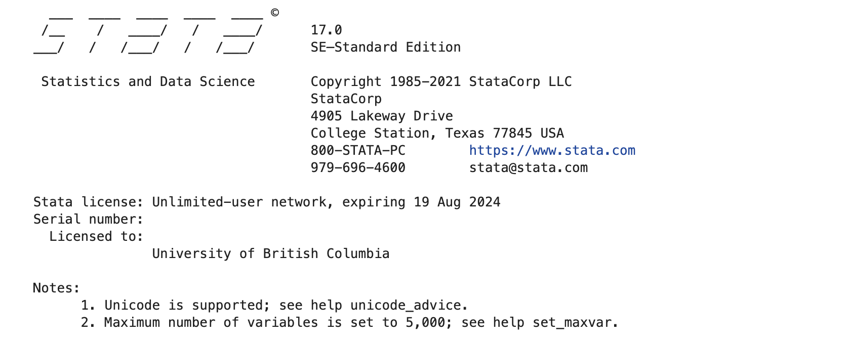
Before we begin, we will need to have installed Stata from the UBC portal. Please be certain to sign in using your CWL before searching for Stata. This software is free for all students in the UBC Faculty of Arts.

We will also need to install Anaconda Navigator in order to be able to run our files in a local version of Jupyter Notebook.

Conda is an open-source package and environment management system. With Conda, we can create a particular directory folder (also known as environment) that will contain the packages that allow us to run Jupyter online notebooks. These notebooks run code coming from different softwares (henceforth referred as kernels): Stata, R, Python, etc. The bare minimum for our environments is some version of Python.

The only way to set up an environment based on Stata requires us to manually connect our computer’s Stata program to Jupyter Notebook.

Note: We only have to do this once on any computer. After that we can go directly to Jupyter Notebooks for our work.

1.2 Setting Up Our Computer

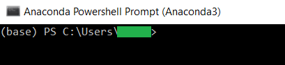
In order to execute the following commands on our computer, we will need to access our computer’s terminal window. A terminal window includes a prompt that indicates where we enter commands. The prompt we see depends on our own system, but it often includes the name of the host we are logged in to, our current working folder, our user name, and a prompt symbol.

To open the terminal in Windows, do one of the following:

1. If you are on Windows 11, click the Start button and select “All Apps”. Scroll down the Start menu and right-click on the file named “Anaconda3 (64-bit)”. Next, left-click on “Anaconda Prompt”, select “more” and click “Run as Administrator”.
2. Alternatively, click the Search icon, start typing “Anaconda Prompt”, and then Run as Administrator from the search results.

Anaconda Location

Once we have the terminal open, we can run the conda commands that find packages to install. This is not dissimilar to downloading software from a server. We want to make sure that the computer first finds the conda-forge channel which contains packages. To allow this, we must run the following commands directly in our own terminal window in Jupyter Notebooks:

conda config --add channels conda-forge
conda config --set channel_priority strict

The goal here is to create a package bundle, i.e. an environment, where we will install some version of R, Stata Kernel, and Jupyter. You can explore the things you can download to an environment from the conda-forge channel by running, for example, conda search r-base, conda search stata_kernel, etc. That way, you can see all the different versions of these packages that you can download from the different channels.

Now we are ready to create a new environment where we can install all these packages. In this particular case, we will create an environment based on Python 3.9.7. Let us create an environment called econ_pystata by writing:

conda create -n econ_pystata python=3.9.7

If we omit the =3.9.7 part, we will create an environment with the default Python version.

We want anything that we install from the channel to be part of this new environment. To do so, we need to activate it by running

conda activate econ_pystata

Now that our environment is activated, we can install everything we want. We begin by installing Jupyter, which will allow us to run the interactive notebooks:

conda install jupyter

1.3 Setting up the STATA Path

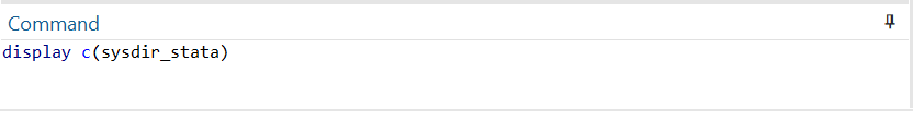
Next, we need to find out where STATA is configured on our computer. To do this, we will first launch STATA. Once it has launched, we will type display c(sysdir_stata) in the command window:

display c(sysdir_stata)

Hit “enter”, and a computer path result should appear in the output above the command window. Write down this path.

STATA path

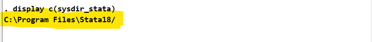
For example, in the remainder of this notebook we will be using the default path for STATA 18 on Windows 11, which is C:\Program Files\Stata18

1.4 Installing PyStata on Our Environment

To allow Python to find Stata’s installation path and the pystata package, we use the pystata Python module stata_setup.

The simplest way to install this setup module is to use the Python package manager pip from the Python Package Index (PyPI). Open up your Anaconda prompt as an administrator, and activate your environment by typing conda activate econ_pystata.

Then, install the new software by typing the following line of code, and press enter:

pip install --upgrade --user numpy pandas ipython

This will install the required dependencies for the pystata package.

Now, we are ready to install the package. Type the following line of code in your anaconda prompt:

pip install --upgrade --user stata_setup

This will install the stata_setup module.

Note: Whenever you are using pip, make sure that you are running the anaconda prompt as an administrator. Otherwise, this will not work!

1.5 Opening Jupyter Lab

We are now ready to open Jupyter Lab! In your Anaconda navigator, type the following line of code and press enter to open Jupyter lab:

jupyter lab

After a second or two this will open up Jupyter Lab on your web browser. Make sure you are still in the econ_pystata environment!

1.6 Importing Stata into Jupyter

In your notebook, begin by creating a new cell and typing the following two lines of code:

import stata_setup

stata_setup.config('C:\Program Files\Stata18/','se')

The stata_setup.config() function is used to locate STATA through Jupyter. This function has two arguments: the first one is Stata’s installation path and the second one is the edition to use. UBC offers students free access to the Stata SE edition, so make sure your Stata version is Stata SE. If you have a different path to Stata, replace the provided path with your absolute path (Ex. C:\Desktop\Stata18/'). This path should be the one you wrote down above, in Step 1.3.

Pystata Output

We are now ready to start using STATA in Jupyter. Remember to launch your environment and Jupyter Lab again when you want to use Jupyter; you will need to do that part every time. However, you don’t have to install pystata or perform these set-up tasks again.

References

Stata installation for python