# A Code cell looks like this and can execute computations! Press Shift+Enter to compute the operation.
2 + 20.1 - Introduction to JupyterNotebooks
introduction
econ intro
jupyter
basics
getting started
notebooks
troubleshooting
cells
Welcome to COMET! This is the very first notebook most of you will do, and it introduces you to some basics of Jupyter and using this project. Have fun!
Outline
Prerequisites
- None!
Outcomes
This notebook is an introduction to JupyterNotebooks. After completing this notebook, you will be able to:
- Describe the structure of a JupyterNotebook and the role of different kinds of cells
- Understand the relationship between a notebook, the editor, the kernel and output
- Understand the directory structure of a JupyterHub and its relation to your notebook
- Write, edit, and execute code in a JupyterNotebook
- Write, edit, and view text in a Jupyter notebook
- Develop basic troubleshooting skills to use when facing technical challenges with JupyterNotebooks
- Export Jupyter notebooks to other standard file types (e.g.,
.html,.pdf)
References
This notebook is informed by the following sources which are great tools to check out if you’re interested in furthering your knowledge of Notebooks and Data Science best practices more broadly.
Part 1: Introduction to Jupyter
In this notebook we’ll be learning about what JupyterNotebooks are and how they work. If you’re reading this, you’re already connected to a Notebook and are one step closer to becoming a Jupyter expert! Notebooks are easily accessed through JupyterHub, which is a web-based interactive integrated development environment (IDE) typically maintained by an organization or institution. These hubs often have different software and tools for collaboration preconfigured for students like you to use. Both JuptyerHub and JupyterNotebooks stem from Jupyter, which is a connected system of open-source tools designed to support interactive, web-based computing (jupyter.org).
In this Notebook, we will specifically be using JupyterLab; the classic interface is similar, but you may notice some labeling differences.
Throughout the COMET Jupyter Notebooks, we’ll bring together theoretical learning instruction, hands-on coding opportunities and automatic feedback to create a comprehensive learning environment. You’ll also notice sections like this:
🔎 Let’s think critically
🟠 Some critical questions or
🟠 Context will go here!
These sections will invite you to pause and reflect on your learning through different lenses. We invite you to think about the series of critical questions or context presented in those sections - bonus points if you also discuss with your peers! Happy learning!
Key Terms
Below are a few key terms that define and contextualize components of the technical environment which Jupyter operates in. As you work through this notebook, try to identify the various (largely invisible) processes and infrastructures that enable you to read the contents of this notebook, run code cells and write text in the notebook, among other things.
- An Integrated Development Environment (IDE) is a type of software application that can be used to work on coding tasks. JupyterHub is an IDE that works really well for collaborative econometric analyses because it contains various features that allow users to write, upload, co-develop and give feedback on files.
- Open source is a copyright term which refers to a source code that is made freely available for modification and sharing. Jupyter and JupyterNotebooks are an example of an open source project because anyone can access the code and documentation used to make them.
- Cloud based describes any computing services or resources that rely on the internet to function. If you are reading this notebook in a browser, for example, your device has used an internet protocol to request access to this notebook from the server that stores this notebook (the server said yes!)
- The Client-server relationship is the underlying relationship that allows the internet to exist as we know it. Client refers to the computer asking for information on the internet and server refers to the computer that responds to requests.
- A Kernel is an execution environment which connects Notebooks with programming languages in order to allow code (written in R or Python, for example) to be executed in the Notebook. Clients (you) can send instructions to a kernel to perform operations on data.
For example, when the operation \(1+1\) is typed into a JupyterNotebook, the web browser (that you are viewing the notebook in) sends a request to the kernel (for this notebook, the R kernel is being used) which computes the request and sends the answer back to your notebook, producing the result: \(2\).
One final term to consider as you begin using notebooks for econometrics is reproducibility. Reproducibility is a core priority in empirical economics and data science. It means ensuring the creation of analyses that can reliably reproduce the same results when analyzing the same data at a later time; reproducibility is a key component of the scientific method. Notebooks allow us to write executable code, attach multimedia and leave meaningful text annotations and discussion throughout our analysis, all of which contribute to a reproducible and transparent data workflow.
🔎 Let’s think critically
🟠 How might the two concepts of open source and accessibility be connected?
🟠 Who might benefit from econometrics analyses that are reproducible?
Cells
Notebooks are composed of different types of cells. The most common types we will work with are Code and Markdown cells.
Running a code cell can be done in a few different ways, but the most common are:
- Selecting the cell you wish to run and pressing
Shift + Enteron your keyboard - Selecting the cell you wish to run and clicking the Run button in the menu above the worksheet (this button looks like a standard “play” button)
Do you see the answer appear below the cell? Cells can include many things, including very complicated operations. Try running the next cell:
source("getting_started_intro_to_jupyter_tests.r")This cell executed a script called testing_intro_to_jupyter.r that, among other things, printed that text. However, cells can contain things other than just code. In fact, we’ve been reading cells all along!
When you double click on this current cell, you can see what a Markdown cell looks like and how it can hold formatted text such as:
- lists,
- mathematical variables like \(x\) and \(y\),
- links like this one to the Jupyter Homepage (jupyter.org)!
Markdown is a simple plain text language that uses a basic syntax to add features like bold and italics to text.
- adding two asterisks ** on either side of a word or phrase makes it bold
- adding one underscore _ on either side of a word or phrase makes it italicized
There are many other types of formatting that Markdown supports.
Note: Social platforms like Discord, Facebook, Twitter and LinkedIn also use the Markdown language to add flavour to text! You can learn more about the features of the Markdown language on your own by checking out this Markdown Cheatsheet.
Self Tests
One of the most useful features of notebooks is the opportunity to get immediate feedback on your work using tests that are built into particular cells by your instructor. Correct answers produce a "Success!" message while incorrect answers produce a "Solution is incorrect" message. Always be sure to read through test questions carefully because notebooks are not very forgiving when it comes to uppercase/lowercase mix-ups, typos or unspecified spaces between words. Time for some practice!
# What country is the University of British Columbia in?


# Replace ... with your answer to the following question
# Be sure to use uppercase for the first letter and keep the ""

answer_1 <- "..."

test_1()
Now try this one:
# What is 2 + 2?


# Replace ... with your answer
# Your answer should be a single digit

answer_2 <- ...

test_2()
Running Code
After using Shift + Enter or pressing the Run button, we are able to tell if a code cell is running by looking at the kernel symbol at the top right of our window. When the symbol is empty, the kernel is not busy and is ready to execute code. When the symbol is filled in, the kernel is busy executing code. When we are executing a simple operation, the kernel symbol will usually flicker on for a brief moment before turning off again. When we are executing a series of complex operations or loading a large data set, the kernel may be filled in for longer as it has to work harder to perform these operations.
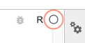
Kernel is not running
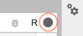
Kernel is running
# When a kernel is filled in, is it (A) running or (B) not running?


# Replace ... with the answer: "A" or "B"
# Be sure to use uppercase letters and keep the ""

answer_3 <- "..."

test_3()
There are a few other kernel images that can occur (like a bomb) which indicate that the kernel has crashed or been disconnected; they usually mean your notebook has encountered a problem and you need to refresh the page.
Things to watch out for
When a code cell is run, it will execute all of the code contained in the cell and produce an output (if applicable) directly below the particular code cell being run. Outputs can include printed text or numbers, data frames and data visualizations. Code cells can be run individually or as a group; we can even run the entirety of a Notebook depending on which command you select in the Run menu in Jupyter.
The most important principle to remember for Jupyter is that the order in which cells are written and run in matters.
What does this mean?
Notebooks are typically written to be executed from top to bottom in a linear fashion. Running all cells from top to bottom can be achieved by going to Run > Run All Cells in the menu. When cells are run in a non-linear order, however, Jupyter can get confused and render objects in unintended ways.
Let’s see an example of how this can create unexpected results.
Try running these cells in the following orders
- cell 1, cell 2, cell 3
then try
- cell 2, cell 1, cell 3
#cell 1: assigns object_a the value 2+2
object_a <- 2+2
#cell 2: assigns object_a the value 1+2
object_a <- 1+2#cell 3: prints object_a
object_aAs you may have noticed, different values are assigned to object_a in different code cells. The kernel will always use the most recent value that has been assigned to object_a, which is why different values are printed in cell 3 depending on the order in which cells 1 and 2 are run.
The rule of thumb, then, is to always write and execute code from the start to the finish so as to avoid any discrepancies.
Part 2: Working with the Jupyter files
Directories
Notebooks are stored in directories in JupyterHub. It can be helpful to think about JupyterHub as an actual hub - that is, a place where different hub users (holding individual Jupyter accounts) can gather to share and collaborate on files. Directories store files in a similar way that a folder on our computer does. The only difference is, with JupyterHub, the cloud-based format allows directories to be used either individually or collaboratively. The directory browser is located on the left hand side of the notebook interface and can be used to store other files including:
- Images
- Data Files
- Other Code files
- etc.
# In one word, where are Notebooks stored?

# Replace ... with your answer
# Be sure to use lowercase letters and keep the ""

answer_4 <- "..."

test_4()
By default, when we use a function that requires a file, Jupyter will look in the notebook’s directory, unless specified otherwise.

The image above is visualized in the notebook by calling a pre-loaded image from the directory into the Notebook using the following instructions:

See if you can spot the
welcome_to_jupyter.pngfile in this notebook’s directory under: “media”
Troubleshooting
Sometimes Notebooks are not run from start to finish or other things go awry which can produce an error. If you are ever in this situation, one of the first things to do is select the Kernel > Restart Kernel and Run All Cells function. This will restart the Notebook session and will clear the Notebook’s “memory” from all objects and commands that have been previously run.
If you run into a situation where your kernel is stuck (i.e., it is filled in) for a very long time, you can also try these fixes:
- At the top of your screen, click Kernel, then Interrupt Kernel.
- If that doesn’t help, click Kernel, then Restart Kernel… If you do this, you will have to run your code cells from the start of your notebook up until where you paused your work.
- If that still doesn’t help, restart Jupyter. First, save your work by clicking File at the top left of your screen, then Save Notebook. Next, if you are accessing Jupyter using a JupyterHub server, from the File menu click Hub Control Panel. Choose Stop My Server to shut it down, then the Start My Server button to start it back up. If you are running Jupyter on your own computer, from the File menu click Shut Down, then start Jupyter again. Finally, navigate back to the notebook you were working on.
- If none of these things work, speak to your TA or instructor about the issue.
Exporting
Notebooks automatically save our work as we write and edit our document. When we are ready to export our file, we can choose from a few different output formats including: .html, .pdf and Jupyter’s own .ipynb (which is a more readable form of a .json file). Be sure you export your files in the format specified by your instructor!
To export your file, go to File > Save and Export As… > Then select your format of choice and save the file with an intuitive name that describes its contents.
Test your knowledge
A few notes about writing your own Notebooks:
- Cells can be added to notebooks (when the cell is selected, indicated by a blue highlight on the left hand side) by using the
+arrow near the top right of the window (not the blue button). Alternatively, you can use theakey to add a cell above your current cell, andbto add a cell below your current cell. - Cells can be deleted by right-clicking on the cell and selecting Delete Cells. Alternatively, you can double click the
dkey to delete a current cell. - A cell’s status (as either a code or markdown cell) is always indicated and can be changed in the dropdown bar of the menu.
Note: Regarding keyboard shortcuts: keys will do different things depending on which mode you are in. Editing mode lets you edit cells, in which case hitting the
akey will type the letter a. Command mode will let you control JupyterLab, in which case hitting theakey will insert a new cell. You can switch between these modes by hittingEscorEnter.
You can also view a list of all of the different keyboard commands available under the Settings > Advanced Settings Editor in the Settings menu, then selecting Keyboard Shortcuts.
Try executing the following tasks:
- Add a markdown cell below that says: “I can make markdown cells!”
- Add a markdown cell above that contains the previous message, but this time, in italics.
- Add a code cell below that operates the equation \(2\) * \(3\).
- Add a code cell below that assigns the value \(4\) to an object titled
object_1.
Note: you can use the following formula to assign a number or operation to an object:
object_name <- # or equation. When you are working with numbers, you don’t need to attach “” as we did above with text answers.
- Add a code cell below that assigns the value \(10\) to an object titled
object_2. - Add a code cell below to see what happens when you compute:
object_1 + object_2.