4.4 - Advanced - Word Embeddings (R)

advanced

natural language processing

large language models

word embeddings

word2vec

vectors

cosine similarity

This notebook introduces the concept and implementation of word embeddings, as used in AI tools like LLMs, in R.

R Version

This notebook was prepared by Laura Nelson in collaboration with UBC COMET team members: Jonathan Graves, Angela Chen and Anneke Dresselhuis

Prerequisites

Some familiarity programming in R
Some familarity with natural language processing
No computational text experience necessary!

Learning outcomes

In the notebook you will

Familiarize yourself with concepts such as word embeddings (WE) vector-space model of language, natural language processing (NLP) and how they relate to small and large language models (LMs)
Import and pre-process a textual dataset for use in word embedding
Use word2vec to build a simple language model for examining patterns and biases textual datasets
Identify and select methods for saving and loading models
Use critical and reflexive thinking to gain a deeper understanding of how the inherent social and cultural biases of language are reproduced and mapped into language computation models

Outline

The goal of this notebook is to demystify some of the technical aspects of language models and to invite learners to start thinking about how these important tools function in society.

In particular, this notebook explores features of word embeddings produced through the word2vec model. The questions we ask in this lesson are guided by Ben Schmidt’s blog post, Rejecting the Gender Binary.

The primary corpus we will use consists of the 150 English-language novels made available by the .txtLab at McGill University. We also look at a Word2Vec model trained on the ECCO-TCP corpus of 2,350 eighteenth-century literary texts made available by Ryan Heuser. (Note that the number of terms in the model has been shortened by half in order to conserve memory.)

Key Terms

Before we dive in, feel free to familiarize yourself with the following key terms and how they relate to each other.

Artificial Intelligence (AI): This term is a broad category that includes the study and development of computer systems that can mimic intelligent human behavior (adapted from Oxford Learners Dictionary).

Machine Learning (ML): This is a branch of AI that uses statistical methods to imitate the way that humans learn (adapted from IBM).

Natural Language Processing (NLP): This is a branch of AI that focuses on training computers to interpret human text and spoken words (adapted from IBM).

We note that NLP is a subset of ML in general: Machine Learning is a broader field focused on developing algorithms that allow computers to learn from data and make decisions or predictions without being explicitly programmed for each specific task. Natural Language Processing is a subfield of ML that specifically deals with enabling computers to understand, interpret, and generate human language.

Word Embeddings (WE): this is an NLP process through which human words are converted into numerical representations (usually vectors) in order for computers to be able to understand them (adapted from Turing) This topic is the focus of this notebook.

word2vec: this is an NLP technique that is commonly used to generate word embeddings. It learns vector representations of words by training on various texts, mapping words with similar contexts to similar vectors in a high-dimensional vector space. It uses either the Continuous Bag of Words (CBOW) or Skip-gram architecture to predict words based on their neighbors capturing semantic relationships between words (don’t worry about these words yet, we will learn them later!).

What are Word Embeddings?

Building off of the definition above, word embeddings are one way that humans can represent language in a way that is legible to a machine. More specifically, they are an NLP approach that use vectors to store textual data in multiple dimensions; by existing in the multi-dimensional space of vectors, word embeddings are able to include important semantic information within a given numeric representation.

For example, if we are trying to answer a research question about how popular a term is on the web at a given time, we might use a simple word frequency analysis to count how many times the word “candidate” shows up in tweets during a defined electoral period. However, if we wanted to gain a more nuanced understanding of what kind of language, biases or attitudes contextualize the term, “candidate” in discourse, we would need to use a method like word embedding to encode meaning into our understanding of how people have talked about candidates over time. Instead of describing our text as a series of word counts, we would treat our text like coordinates in space, where similar words and concepts are closer to each other, and words that are different from each other are further away.

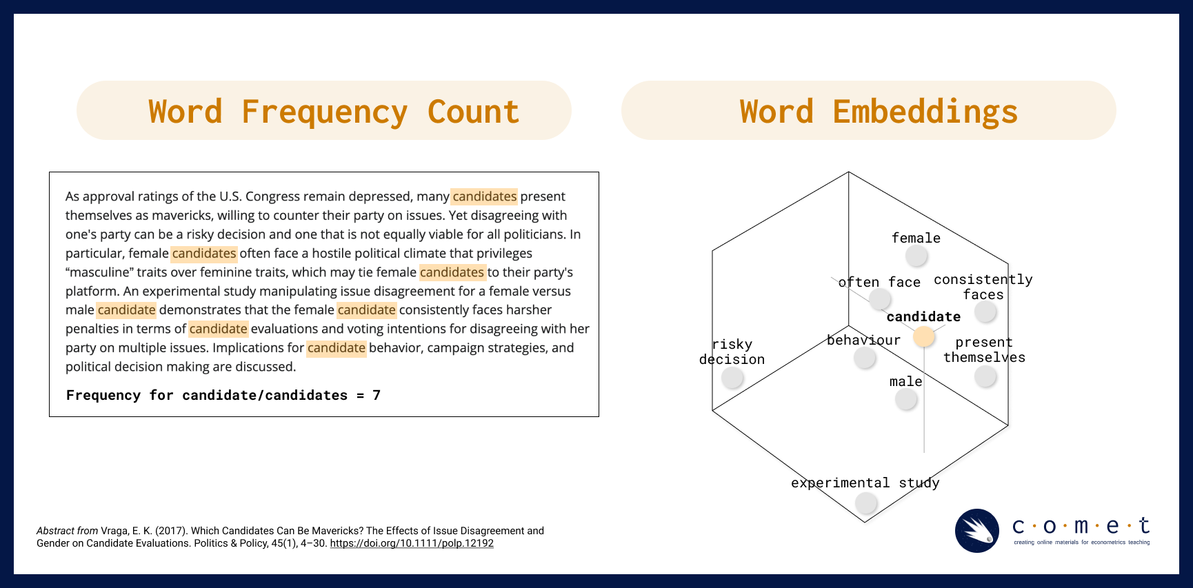
Comparing word frequency count and word embedding methods

For example, in the visualization above, a word frequency count returns the number of times the word “candidate” or “candidates” is used in a sample text corpus. When a word embedding is made from the same text corpus, we are able to map related concepts and phrases that are closely related to “candidate” as neighbours, while other words and phrases such as “experimental study” (which refers to the research paper in question, and not to candidates specifically) are further away.

Here is another example of how different, but related words might be represented in a word embedding:

Word embeddings in action: Kaveh-Yazdy & Zarifzadeh (2021)

In their 2021 paper “Measuring Economic Policy Uncertainty Using an Unsupervised Word Embedding-based Method”, Fatemeh Kaveh-Yazdy and Sajjad Zarifzadeh introduce a novel approach to measure Economic Policy Uncertainty (EPU), a measure of the level of economic uncertainty caused by new economic policies made by governments. By analyzing news data with a word embedding-based method and a dataset of 10 million Persian news articles, the authors constructed a Persian EPU index. The authors found a significant alignment between this EPU index and significant economic and political events in Iran at the time, matching trends in the global World Uncertainty Index (WUI). Additionally, the proposed method showed a strong correlation between suicide rates and EPU, particulary noting a higher correlation relative to other traditional EPU indices, supporting its reliability in reflecting societal impacts of economic uncertainty (Kaveh-Yazdy & Zarifzadeh, 2021).

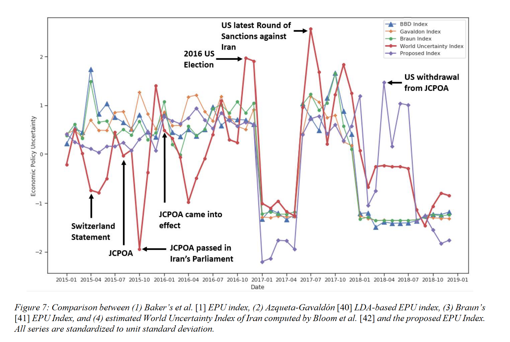
Kaveh-Yazdy & Zarifzadeh's results showing a strong overlap between word-embedding EPU and traditional EPU
A graph from Kaveh-Yazdy & Zarifzadeh (2021) showcasing their word embedding-based EPU calculation compared to traditional EPU

A Brief Review of Vectors

Vectors in 2d and 3d
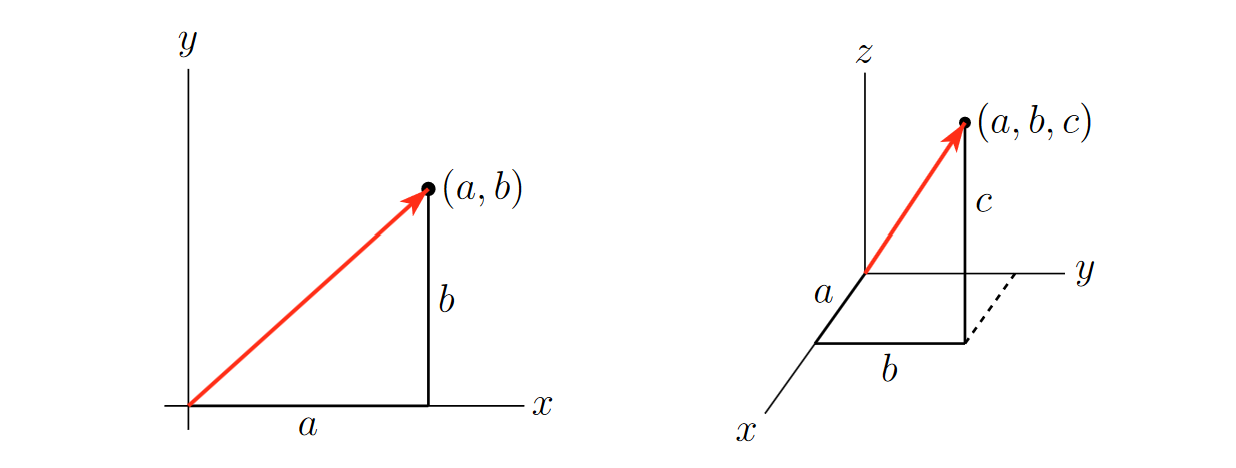
Vectors in $\mathbb{R}^2$ and $\mathbb{R}^3$, courtesy of CLP3

A vector is a mathematical object that has both a magnitude and a direction. You can think of it as an arrow pointing from one location to another in space. This arrow represents both a size (how long it is) and a direction (the way it’s pointing).

The vectors used in this notebook, for the purposes of learning, are two dimensional: they exist in $ ^2$. However, real embeddings are always multidimensional (we will get back to why this is the case later): they exist in $\mathbb{R}^n$, where $n$ is some verly large number.

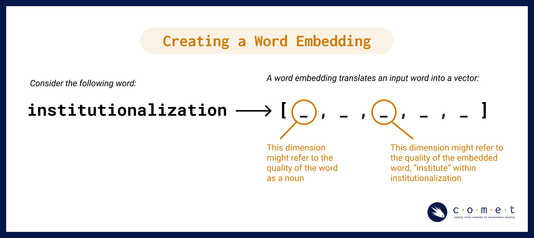
Making a Word Embedding

So, how do word embeddings work? To make a word embedding, an input word gets compressed into a dense vector.

Creating a word embedding vector

The magic and mystery of the word embedding process is that often the vectors produced during the model embed qualities of a word or phrase that are not interpretable by humans. However, for our purposes, having the text in vector format is all we need. With this format, we can perform tests like cosine similarity (which we will discuss later) and other kinds of operations. Such operations can reveal many different kinds of relationships between words, as we’ll examine a bit later.

Word2vec and vector encoding

The simplest form of vector-word encoding is called one-hot encoding. One-hot encoding is very similar to the creation of dummy varibles for categorical data in linear regressions: each word in the english language is assigned a binary value in a vector in $\mathbb{R}^k$, where $k$ is the number of words in the english language. For example, consider a language with only three words in it: “cat”, “dog”, and horse. Hence, our vector encodings are:

\[\text{Cat} \to <1,0,0>\] \[\text{Dog} \to <0,1,0>\] \[\text{Horse} \to <0,0,1>\]

Naturally, this becomes unfeasable with real languages: The english language contains roughly 1 million words, meaning each vector would be 1-million-dimensional, and each vector would require 4MB of storage on your computer. Good luck working with that!

This is where Word2Vec comes in: Word2Vec is a ML model designed to represent words as vectors that capture semantic relationships. It generates low-dimensional word embeddings by learning from word contexts in a large corpus, allowing words with similar meanings to have vectors close together. More precisely, word2vec is an algorithmic learning tool rather than a specific neural net that is already trained. The example we will be working through today has been made using this tool. - Unlike one-hot encodings, where words are represented in a high-dimensional space equal to the size of the vocabulary (potentially tens of thousands of dimensions) embeddings have values in every dimension, allowing them to be compact and memory-efficient, meaning that word embeddings usually have only 100-300 dimensions. This reduction captures essential semantic information without excessive dimensionality.

The series of algorithms inside of the word2vec model try to describe and acquire parameters for a given word in terms of the text that appear immediately to the right and left in actual sentences. Essentially, it learns how to predict text.

Without going too deep into the algorithm, suffice it to say that it involves a two-step process:

First, the input word gets compressed into a dense vector, as seen in the simplified diagram, “Creating a Word Embedding,” above.
Second, the vector gets decoded into the set of context words. Keywords that appear within similar contexts will have similar vector representations in between steps.

Imagine that each word in a novel has its meaning determined by the ones that surround it in a limited window. For example, in Moby Dick’s first sentence, “me” is paired on either side by “Call” and “Ishmael.” After observing the windows around every word in the novel (or many novels), the computer will notice a pattern in which “me” falls between similar pairs of words to “her,” “him,” or “them.” Of course, the computer had gone through a similar process over the words “Call” and “Ishmael,” for which “me” is reciprocally part of their contexts. This chaining of signifiers to one another mirrors some of humanists’ most sophisticated interpretative frameworks of language.

The two main model architectures of word2vec are Continuous Bag of Words (CBOW) and Skip-Gram, which can be distinguished partly by their input and output during training.

CBOW takes the context words (for example, “Call”,“Ishmael”) as a single input and tries to predict the word of interest (“me”).

Skip-Gram does the opposite, taking a word of interest as its input (for example, “me”) and tries to learn how to predict its context words (“Call”,“Ishmael”).

In general, CBOW is is faster and does well with frequent words, while Skip-Gram potentially represents rare words better.

Since the word embedding is a vector, we are able perform tests like cosine similarity (which we’ll learn more about in a bit!) and other kinds of operations. Those operations can reveal many different kinds of relationships between words, as we shall see.

Bias and Language Models

You might already be piecing together that the encoding of meaning in word embeddings is entirely shaped by patterns of language use captured in the training data. That is, what is included in a word embedding directly reflects the complex social and cultural biases of everyday human language - in fact, exploring how these biases function and change over time (as we will do later) is one of the most interesting ways to use word embeddings in social research.

It is simply impossible to have a bias-free language model (LM).

In LMs, bias is not a bug or a glitch, rather, it is an essential feature that is baked into the fundamental structure. For example, LMs are not outside of learning and absorbing the pejorative dimensions of language which in turn, can result in reproducing harmful correlations of meaning for words about race, class or gender (among others). When unchecked, these harms can be “amplified in downstream applications of word embeddings” (Arseniev-Koehler & Foster, 2020, p. 1).

Just like any other computational model, it is important to critically engage with the source and context of the training data. One way that Schiffers, Kern and Hienert suggest doing this is by using domain specific models (2023). Working with models that understand the nuances of your particular topic or field can better account for “specialized vocabulary and semantic relationships” that can help make applications of WE more effective.

Preparing for our Analysis

Word2vec Features

Here are a few features of the word2vec tool that we can use to customize our analysis:

size: Number of dimensions for word embedding model
window: Number of context words to observe in each direction
min_count: Minimum frequency for words included in model
sg (Skip-Gram): ‘0’ indicates CBOW model; ‘1’ indicates Skip-Gram
alpha: Learning rate (initial); prevents model from over-correcting, enables finer tuning
iterations: Number of passes through dataset
batch size: Number of words to sample from data during each pass

Note: the script uses default value for each argument.

Some limitations of the word2vec Model

Within word2vec, common articles or conjunctions, called stop words such as “the” and “and,” may not provide very rich contextual information for a given word, and may need additional subsampling or to be combined into a word phrase (Anwla, 2019).
Word2vec isn’t always the best at handling out-of-vocabulary words well (Chandran, 2021).

Let’s begin our analysis!

Exercise #1: Eggs, Sausages and Bacon

To begin, we are going to install and load a few packages that are necessary for our analysis. Run the code cells below if these packages are not already installed:

# uncomment these by deleting the "#" to install them

#install.packages("tidyverse")
#install.packages("repr")
#install.packages("proxy")
#install.packages("scales")
#install.packages("tm")
#install.packages("MASS")
#install.packages("SentimentAnalysis")
#install.packages("reticulate")
#install.packages("plotly")

# Load the required libraries
library(tidyverse)
library(repr)
library(proxy)
library(tm)
library(scales)
library(MASS)
library(plotly)


# Set up figures to save properly
options(jupyter.plot_mimetypes = "image/png")

# Time: 30s
library(reticulate)
gensim <- import("gensim")

Create a Document-Term Matrix (DTM) with a Few Pseudo-Texts

To start off, we’re going to create a mini dataframe called a Document-Term Matrix (DTM). A DTM is a matrix (or in our case, a tidyverse dataframe) that represents the frequency of terms (words) appearing in a collection of documents. Our DTM is based on the use of the words “eggs,” “sausages” and “bacon” found in three different novels: A, B and C.

# Construct dataframe
columns <- c('eggs', 'sausage', 'bacon')
indices <- c('Novel A', 'Novel B', 'Novel C')
dtm <- data.frame(eggs = c(50, 90, 20),
                  sausage = c(60, 10, 70),
                  bacon = c(60, 10, 70),
                  row.names = indices)

# Show dataframe
print(dtm)

Visualize

We’ll start by graphing all three axes using the plotly library:

library(plotly)

fig <- plot_ly(data = dtm, x = ~sausage, y = ~eggs, z = ~bacon,
  type = "scatter3d", mode = "markers+text", marker = list(size = 5), text = rownames(dtm), 
  textposition = "top right", hoverinfo = "text")

fig <- fig |> layout(
  scene = list(xaxis = list(title = 'Sausage'), yaxis = list(title = 'Eggs'), zaxis = list(title = 'Bacon')), title = "3D Plot of Books by Sausage, Eggs, and Bacon Counts")

fig

Now, let’s take a look at just two axes, eggs and sausage.

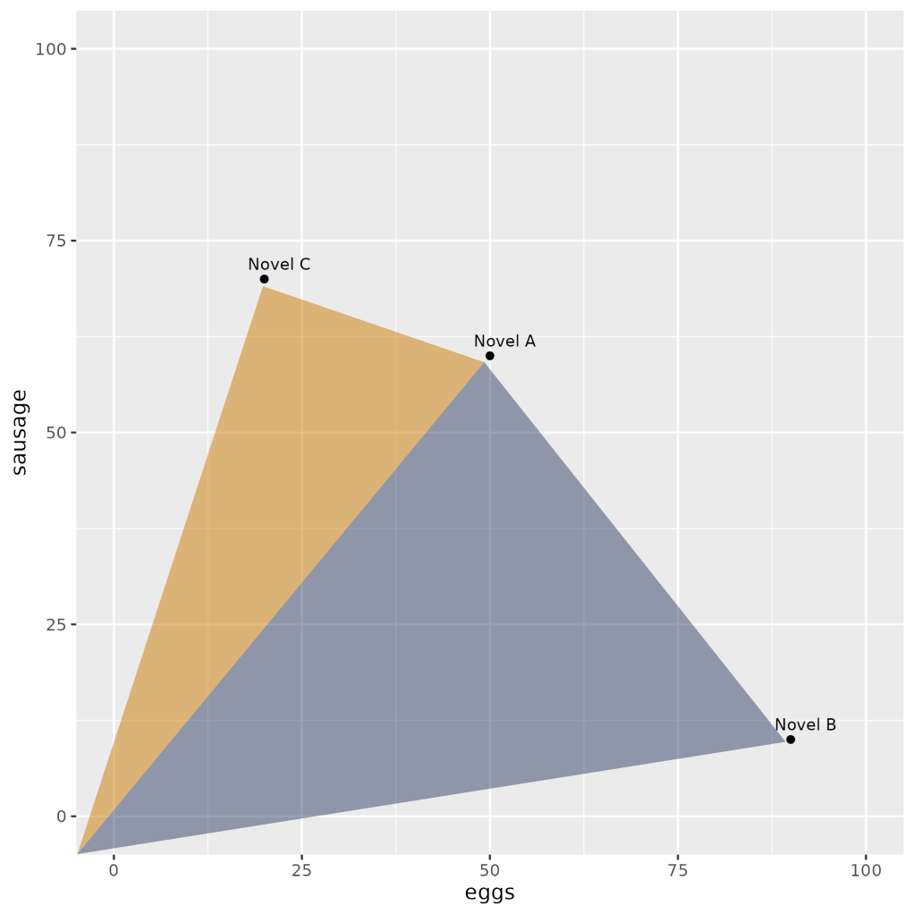
ggplot(dtm, aes(x = eggs, y = sausage)) +
  geom_point() +
  geom_text(aes(label = rownames(dtm)), nudge_x = 2, nudge_y = 2, size = 3) +
  xlim(0, 100) +
  ylim(0, 100) +
  labs(x = "eggs", y = "sausage")

A Return to Vectors

At a glance, a couple of points are lying closer to one another. We used the word frequencies of just two words in order to plot our texts in a two-dimensional plane. The term frequency “summaries” of Novel A & Novel C are pretty similar to one another: they both share a major concern with “sausage”, whereas Novel B seems to focus primarily on “eggs.”

This raises a question: how can we operationalize our intuition that spatial distance expresses topical similarity?

Cosine Similarity

The most common measurement of distance between points is their Cosine Similarity. Cosine similarity can operate on textual data that contain word vectors and allows us to identify how similar documents are to each other, for example. Cosine Similarity thus helps us understand how much content overlap a set of documents have with one another. For example, imagine that we were to draw an arrow from the origin of the graph - point (0,0) - to the dot representing each text. This arrow is called a vector.

Mathematically, this can be represented as:

Using our example above, we can see that the angle from (0,0) between Novel C and Novel A (orange triangle) is smaller than between Novel A and Novel B (navy triangle) or between Novel C and Novel B (both triangles together).

Because this similarity measurement uses the cosine of the angle between vectors, the magnitude is not a matter of concern (this feature is really helpful for text vectors that can often be really long!). Instead, the output of cosine similarity yields a value between 0 and 1 (we don’t have to work with something confusing like 18º!) that can be easily interpreted and compared - and thus we can also avoid the troubles associated with other dimensional distance measures such as Euclidean Distance.

Kaveh-Yazdy & Zarifzadeh (2021)

In their paper, Kaveh-Yazdy & Zarifzadeh measure EPU by embedding various persian news articles into a tri-axis, two dimensional representation system:

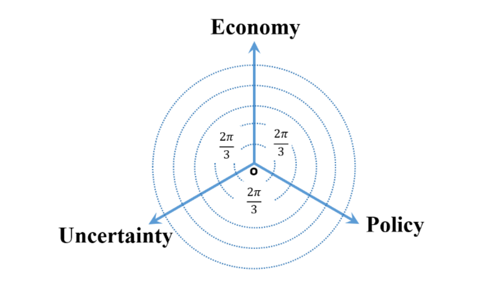
This Tri-axial Representation System is a non-standard coordinate system used to map the similarity values of news articles with respect two three categories: Economy, Policy, and Uncertainty- within a 2D plane. Introducing a tri-asix system in 2d space instead of a cartesian system in 3d space allows the authors to focus in documents that cover all three categories of EPU at a general level instead of narrowing in on documents that focused on one facet of EPU at a maximal level.

The authors assign weights to each document using cosine similarity, measuring the cosing similairy of the words in each document and the three seed words (Economy, Policy, and Uncertainty). However, to avoid overclouding the data with words that don’t matter much, the authors introduce an additional similarity theshold, where words under said similarity threshold are assigned a similarity value of 0 (Kaveh-Yazdy & Zarifzadeh, 2021).

Calculating Cosine Distance

# Assuming dtm_df is a data frame containing the document-term matrix
dtm_matrix <- as.matrix(dtm)

# Calculate cosine similarity
cos_sim <- proxy::dist(dtm_matrix, method = "cosine")


# Although we want the Cosine Distance, it is mathematically simpler to calculate its opposite: Cosine Similarity
# The formula for Cosine Distance is = 1 - Cosine Similarity

# Convert the cosine similarity matrix to a 2-dimensional array
# So we will subtract the similarities from 1
n <- nrow(dtm_matrix)
cos_sim_array <- matrix(1 - as.vector(as.matrix(cos_sim)), n, n)

# Print the result
print(cos_sim_array)

# Make it a little easier to read by rounding the values
cos_sim_rounded <- round(cos_sim_array, 2)

# Label the dataframe rows and columns with eggs, sausage and bacon
cos_df <- data.frame(cos_sim_rounded, row.names = indices, check.names = FALSE)
colnames(cos_df) <- indices

# Print the data frame
head(cos_df)

Exercise #2: Working with 18th Century Literature

Now that we’ve taken a look at word embeddings using fake data, let’s test out our knowledge on actual literature. We’ll be using a collection of texts from famous authors Jane Austen, Nathaniel Hawthorne, and F. Scott Fitzgerald. These books have already been translated for us into .txt form to make analysis easier. All three authors have uniquely distinct literary styles: Fitzgerald have very lyrical writing, focusing on the american dream, wealth, and desire. Hawthorne’s writings are very symbolic and allegorical, focusing on sin, guilt, morality, and the supernatural. On the other hand, Austen’s prose is elegant and clear, and her writings focus on social class, marriage, and the role of women in society.

We hope that some of these differences will come through in our analysis.

# Load the required libraries
library(tidyverse)
library(repr)
library(proxy)
library(tm)
library(scales)
library(MASS)


# Set up figures to save properly
options(jupyter.plot_mimetypes = "image/png") 

# Time: 3 mins
# File paths and names
filelist <- c(
  'txtlab_Novel450_English/EN_1850_Hawthorne,Nathaniel_TheScarletLetter_Novel.txt',
  'txtlab_Novel450_English/EN_1851_Hawthorne,Nathaniel_TheHouseoftheSevenGables_Novel.txt',
  'txtlab_Novel450_English/EN_1920_Fitzgerald,FScott_ThisSideofParadise_Novel.txt',
  'txtlab_Novel450_English/EN_1922_Fitzgerald,FScott_TheBeautifulandtheDamned_Novel.txt',
  'txtlab_Novel450_English/EN_1811_Austen,Jane_SenseandSensibility_Novel.txt',
  'txtlab_Novel450_English/EN_1813_Austen,Jane_PrideandPrejudice_Novel.txt'
)

novel_names <- c(
  'Hawthorne: Scarlet Letter',
  'Hawthorne: Seven Gables',
  'Fitzgerald: This Side of Paradise',
  'Fitzgerald: Beautiful and the Damned',
  'Austen: Sense and Sensibility',
  'Austen: Pride and Prejudice'
)

# Function to read non-empty lines from the text file
readNonEmptyLines <- function(filepath) {
  lines <- readLines(filepath, encoding = "UTF-8")
  non_empty_lines <- lines[trimws(lines) != ""]
  return(paste(non_empty_lines, collapse = " "))
}

# Read non-empty texts into a corpus
text_corpus <- VCorpus(VectorSource(sapply(filelist, readNonEmptyLines)))

# Preprocess the text data
text_corpus <- tm_map(text_corpus, content_transformer(tolower))
text_corpus <- tm_map(text_corpus, removePunctuation)
text_corpus <- tm_map(text_corpus, removeNumbers)
text_corpus <- tm_map(text_corpus, removeWords, stopwords("english"))
text_corpus <- tm_map(text_corpus, stripWhitespace)

## Time: 5 mins
# Create a custom control for DTM with binary term frequency
custom_control <- list(
  tokenize = function(x) SentimentAnalysis::ngram_tokenize(x, ngmax = 1),
  bounds = list(global = c(3, Inf)),
  weighting = weightTf
)

# Convert the corpus to a DTM using custom control
dtm <- DocumentTermMatrix(text_corpus, control = custom_control)

# Convert DTM to a binary data frame (0 or 1)
dtm_df_novel <- as.data.frame(as.matrix(dtm > 0))
colnames(dtm_df_novel) <- colnames(dtm)

# Set row names to novel names
rownames(dtm_df_novel) <- novel_names

# Print the resulting data frame
tail(dtm_df_novel)

# Just as we did above with the small data frame, we'll find the cosine similarity for these texts
cos_sim_novel <- as.matrix(proxy::dist(dtm_df_novel, method = "cosine"))

# Convert the cosine similarity matrix to a 2-dimensional array
n <- nrow(dtm_df_novel)
cos_sim_array <- matrix(1 - as.vector(as.matrix(cos_sim_novel)), n, n)

# Round the cosine similarity matrix to two decimal places
cos_sim_novel_rounded <- round(cos_sim_array, 2)

# Print the rounded cosine similarity matrix
print(cos_sim_novel_rounded)

# Again, we'll make this a bit more readable
cos_df <- data.frame(cos_sim_novel_rounded, row.names = novel_names, check.names = FALSE)

# Set column names to novel names
colnames(cos_df) <- novel_names

# Print the DataFrame
head(cos_df)

# Transform cosine similarity to cosine distance
cos_dist <- 1 - cos_sim_novel_rounded

# Perform MDS
mds <- cmdscale(cos_dist, k = 2)

# Extract x and y coordinates from MDS output
xs <- mds[, 1]
ys <- mds[, 2]

# Create a data frame with x, y coordinates, and novel names
mds_df <- data.frame(x = xs, y = ys, novel_names = novel_names)

ggplot(mds_df, aes(x, y, label = novel_names)) +
  geom_point(size = 4) +
  geom_text(hjust =0.6, vjust = 0.2, size = 4, angle = 45, nudge_y = 0.01) +  # Rotate text and adjust y position
  labs(title = "MDS Visualization of Novel Differences") +
  theme_minimal() +
  theme(
    plot.title = element_text(size = 20, hjust = 0.6, margin = margin(b = 10)),
    plot.margin = margin(5, 5, 5, 5, "pt"),  # Adjust the margin around the plot
    plot.background = element_rect(fill = "white"),  # Set the background color of the plot to white
    plot.caption = element_blank(),  # Remove the default caption
    axis.text = element_text(size = 12),  # Adjust the size of axis text
    legend.text = element_text(size = 12),  # Adjust the size of legend text
    legend.title = element_text(size = 14)  # Adjust the size of legend title
  )

The above method has a broad range of applications, such as unsupervised clustering. Common techniques include K-Means Clustering and Hierarchical Dendrograms. These attempt to identify groups of texts with shared content, based on these kinds of distance measures.

Here’s an example of a dendrogram based on these six novels:

# Assuming you have already calculated the "cos_dist" matrix and have the "novel_names" vector

# Perform hierarchical clustering
hclust_result <- hclust(as.dist(cos_dist), method = "ward.D")

# Plot the dendrogram
plot(hclust_result, hang = -1, labels = novel_names)

# Optional: Adjust the layout to avoid cutoff labels
par(mar = c(5, 4, 2, 10))  # Adjust margins

# Display the dendrogram plot

Vector Semantics

We can also turn this logic on its head. Rather than produce vectors representing texts based on their words, we will produce vectors for the words based on their contexts.

# Transpose the DTM data frame
transposed_dtm <- t(dtm_df_novel)

# Display the first few rows of the transposed DTM
tail(transposed_dtm)

Because the number of words is so large, for memory reasons we’re going to work with just the last few, pictured above.

If you are running this locally, you may want to try this with more words

# Assuming dtm_df is a data frame containing the document-term matrix
tail_transposed_dtm <- tail(transposed_dtm)

dtm_matrix <- as.matrix(tail_transposed_dtm) #remove 'tail_' to use all words

# Calculate cosine similarity
cos_sim_words <- proxy::dist(dtm_matrix, method = "cosine")

# Convert the cosine similarity matrix to a 2-dimensional array
n <- nrow(dtm_matrix)
cos_sim_words <- matrix(1 - as.vector(as.matrix(cos_sim_words)), n, n)

# Print the result
head(cos_sim_words)

# In readable format

cos_sim_words <- data.frame(round(cos_sim_words, 2))
row.names(cos_sim_words) <- row.names(tail_transposed_dtm) #remove tail_ for all
colnames(cos_sim_words) <- row.names(tail_transposed_dtm) #remove tail_ for all

head(cos_sim_words)

Theoretically we could visualize and cluster these as well - but it would a lot of computational power!

We’ll instead turn to the machine learning version: word embeddings

#check objects in memory; delete the big ones

sort(sapply(ls(), function(x) format(object.size(get(x)), unit = 'auto')))
            
rm(cos_sim_words, cos_sim_array, text_corpus, dtm_df_novel)
            
sort(sapply(ls(), function(x) format(object.size(get(x)), unit = 'auto')))

Exercise #3: Using Word2vec with 150 English Novels

In this exercise, we’ll use an English-language subset from a dataset about novels created by Andrew Piper. Specifically we’ll look at 150 novels by British and American authors spanning the years 1771-1930. These texts reside on disk, each in a separate plaintext file. Metadata is contained in a spreadsheet distributed with the novel files.

Metadata Columns

Filename: Name of file on disk
ID: Unique ID in Piper corpus
Language: Language of novel
Date: Initial publication date
Title: Title of novel
Gender: Authorial gender
Person: Textual perspective
Length: Number of tokens in novel

Import Metadata

# Import Metadata into Dataframe
meta_df <- read.csv('resources/txtlab_Novel450_English.csv', encoding = 'UTF-8')

# Check Metadata
head(meta_df)

Import Corpus

# Set the path to the 'fiction_folder'
fiction_folder <- "txtlab_Novel450_English/"

# Create a list to store the file paths
file_paths <- list.files(fiction_folder, full.names = TRUE)

# Read all the files as a list of single strings
novel_list <- lapply(file_paths, function(filepath) {
  readChar(filepath, file.info(filepath)$size)
})

# Inspect first item in novel_list
cat(substr(novel_list[[1]], 1, 500))

Pre-Processing

Word2Vec learns about the relationships among words by observing them in context. This means that we want to split our texts into word-units. However, we want to maintain sentence boundaries as well, since the last word of the previous sentence might skew the meaning of the next sentence.

Since novels were imported as single strings, we’ll first need to divide them into sentences, and second, we’ll split each sentence into its own list of words.

# Define a regular expression pattern for sentence splitting
sentence_pattern <- "[^.!?]+(?<!\\w\\w\\w\\.)[.!?]"

# Split each novel into sentences
sentences <- unlist(lapply(novel_list, function(novel) {
  str_extract_all(novel, sentence_pattern)[[1]]
}))

first_sentence <- sentences[1]
print(first_sentence)

We are defining a function called fast_tokenize, we will be using this function later when we train the word vector model. See example usage for its feature.

fast_tokenize <- function(text) {
  
  # Remove punctuation characters
  no_punct <- gsub("[[:punct:]]", "", tolower(text))
  
  # Split text over whitespace into a character vector of words
  tokens <- strsplit(no_punct, "\\s+")[[1]]
  
  return(tokens)
}

# Example usage
text <- "Hello, world! This is an example sentence."
tokens <- fast_tokenize(text)
print(tokens)

# Time: 2 mins
# Split each sentence into tokens
# this will take 1-2 minutes

words_by_sentence <- lapply(sentences, function(sentence) {
  fast_tokenize(sentence)
})

# Remove any sentences that contain zero tokens
words_by_sentence <- words_by_sentence[sapply(words_by_sentence, length) > 0]

# Inspect first sentence

first_sentence_tokens <- words_by_sentence[[1]]
print(first_sentence_tokens)

Training

To train the model we can use this code:

# Time: 3 mins
# Train word2vec model from txtLab corpus

model <- gensim$models$Word2Vec(words_by_sentence, vector_size=100L, window=5L, min_count=25L, sg=1L, alpha=0.025, epochs=5L, batch_words=10000L)

However, this is both very slow and very memory instensive. Instead, we will short-cut here to load the saved results instead:

# Load pre-trained model word2vec model from txtLab corpus
model <- gensim$models$KeyedVectors$load_word2vec_format('resources/word2vec.txtlab_Novel150_English.txt')
model$wv <- gensim$models$KeyedVectors$load_word2vec_format('resources/word2vec.txtlab_Novel150_English.txt')

Embeddings

Note: the output here is different than the Python version, even though the model is using the same parameters and same input, which is sentences

This create a 100-dimension representation of specific words in the text corpus. This is a dense vector, meaning all of the valaues are (usually) non-zero.

# Return dense word vector
vector <- model$wv$get_vector("whale")

data.frame(dimension = 1:100, value = vector)

Vector-Space Operations

The key advantage of the word-embedding is the dense vector representations of words: these allow us to do operations on those words, which are informative for learning about how those words are used.

This is also where the connection with LLM is created: they use these vectors to inform predictions about sequences of words (and sentences, in more complex models)

Similarity

Since words are represented as dense vectors, we can ask how similiar words’ meanings are based on their cosine similarity (essentially how much they overlap). gensim has a few out-of-the-box functions that enable different kinds of comparisons.

# Find cosine distance between two given word vectors

similarity <- model$wv$similarity("pride", "prejudice")
similarity

# Find nearest word vectors by cosine distance

most_similar <- model$wv$most_similar("pride")
most_similar

# Given a list of words, we can ask which doesn't belong

# Finds mean vector of words in list
# and identifies the word further from that mean

doesnt_match <- model$wv$doesnt_match(c('pride', 'prejudice', 'whale'))
doesnt_match

Multiple Valences

A word embedding may encode both primary and secondary meanings that are both present at the same time. In order to identify secondary meanings in a word, we can subtract the vectors of primary (or simply unwanted) meanings. For example, we may wish to remove the sense of river bank from the word bank. This would be written mathetmatically as RIVER - BANK, which in gensim’s interface lists RIVER as a positive meaning and BANK as a negative one.

# Get most similar words to BANK, in order
# to get a sense for its primary meaning

most_similar <- model$wv$most_similar("bank")
most_similar

# Remove the sense of "river bank" from "bank" and see what is left

result <- model$wv$most_similar(positive = "bank", negative = "river")

result

Analogy

Analogies are rendered as simple mathematical operations in vector space. For example, the canonic word2vec analogy MAN is to KING as WOMAN is to ?? is rendered as KING - MAN + WOMAN. In the gensim interface, we designate KING and WOMAN as positive terms and MAN as a negative term, since it is subtracted from those.

# Get most similar words to KING, in order
# to get a sense for its primary meaning

most_similar <- model$wv$most_similar("king")
most_similar

# The canonic word2vec analogy: King - Man + Woman -> Queen

result <- model$wv$most_similar(positive = c("woman", "king"), negative = "man")
result

Gendered Vectors

Can we find gender a la Schmidt (2015)? (Note that this method uses vector projection, whereas Schmidt had used rejection.)

# Feminine Vector

result <- model$wv$most_similar(positive = c("she", "her", "hers", "herself"), negative = c("he", "him", "his", "himself"))
result

# Masculine Vector

result <- model$wv$most_similar(positive = c("he", "him", "his", "himself"), negative = c("she", "her", "hers", "herself"))
result

Visualization

# Note: due to some discrepencies between Python and R, this may not be translated exactly
# Dictionary of words in model

key_to_index <- model$wv$key_to_index #this stores the index of each word in the model

head(key_to_index)

# Visualizing the whole vocabulary would make it hard to read

key_to_index <- model$wv$key_to_index

# Get the number of unique words in the vocabulary (vocabulary size)
vocabulary_size <- length(key_to_index)

# Find most similar tokens
similarity_result <- model$wv$most_similar(positive = c("she", "her", "hers", "herself"),
                                           negative = c("he", "him", "his", "himself"),
                                           topn = as.integer(50))  # Convert to integer

# Extract tokens from the result
her_tokens <- sapply(similarity_result, function(item) item[1])

her_tokens_first_15 <- her_tokens[1:15]

# Inspect list
her_tokens_first_15

# Get the vector for each sampled word

for (i in 1:length(her_tokens)){
    
    if (i == 1) { vectors_matrix <- model$wv$get_vector(i) } else {
        vectors_matrix <- rbind(vectors_matrix, model$wv$get_vector(i))
    } 
    
}

# Print the vectors matrix
head(vectors_matrix, n = 5)

# Calculate distances among texts in vector space

dist_matrix <- as.matrix(proxy::dist(vectors_matrix, by_rows = TRUE, method = "cosine"))

# Print the distance matrix
head(dist_matrix, n = 5)

# Multi-Dimensional Scaling (Project vectors into 2-D)


# Perform Multi-Dimensional Scaling (MDS)
mds <- cmdscale(dist_matrix, k = 2)

# Print the resulting MDS embeddings
head(mds)

plot_data <- data.frame(x = mds[, 1], y = mds[, 2], label = unlist(her_tokens))


# Create the scatter plot with text labels using ggplot2
p <- ggplot(plot_data, aes(x = x, y = y, label = label)) +
  geom_point(alpha = 0) +
  geom_text(nudge_x = 0.02, nudge_y = 0.02) +
  theme_minimal()

# Print the plot
print(p)

# For comparison, here is the same graph using a masculine-pronoun vector

# Find most similar tokens
similarity_result <- model$wv$most_similar(negative = c("she", "her", "hers", "herself"),
                                           positive = c("he", "him", "his", "himself"),
                                           topn = as.integer(50))  # Convert to integer

his_tokens <- sapply(similarity_result, function(item) item[1])


# Get the vector for each sampled word

for (i in 1:length(his_tokens)){
    
    if (i == 1) { vectors_matrix <- model$wv$get_vector(i) } else {
        vectors_matrix <- rbind(vectors_matrix, model$wv$get_vector(i))
    } 
    
}

dist_matrix <- as.matrix(proxy::dist(vectors_matrix, by_rows = TRUE, method = "cosine"))
 
mds <- cmdscale(dist_matrix, k = 2)
                     
plot_data <- data.frame(x = mds[, 1], y = mds[, 2], label = unlist(his_tokens))

# Create the scatter plot with text labels using ggplot2
p <- ggplot(plot_data, aes(x = x, y = y, label = label)) +
  geom_point(alpha = 0) +
  geom_text(nudge_x = 0.02, nudge_y = 0.02) +
  theme_minimal()

# Print the plot
print(p)

Questions:

What kinds of semantic relationships exist in the diagram above?

Are there any words that seem out of place?

3. Saving/Loading Models

# Save current model for later use

model$wv$save_word2vec_format('resources/word2vec.txtlab_Novel150_English.txt')

# Load up models from disk

# Model trained on Eighteenth Century Collections Online corpus (~2500 texts)
# Made available by Ryan Heuser: http://ryanheuser.org/word-vectors-1/

ecco_model <- gensim$models$KeyedVectors$load_word2vec_format('resources/word2vec.ECCO-TCP.txt')

# What are similar words to BANK?

ecco_model$most_similar('bank')

# What if we remove the sense of "river bank"?
ecco_model$most_similar(positive = list('bank'), negative = list('river'))

Exercises!

See if you can attempt the following exercises on your own!

## EX. Use the most_similar method to find the tokens nearest to 'car' in either model.
##     Do the same for 'motorcar'.

## Q.  What characterizes these two words inthe corpus? Does this make sense?

model$wv$most_similar("car")

model$wv$most_similar('motorcar')

## EX. How does our model answer the analogy: MADRID is to SPAIN as PARIS is to __________

## Q.  What has our model learned about nation-states?


model$wv$most_similar(positive = c('paris', 'spain'), negative = c('madrid'))

## EX. Perform the canonic Word2Vec addition again but leave out a term:
##     Try 'king' - 'man', 'woman' - 'man', 'woman' + 'king'

## Q.  What do these indicate semantically?

model$wv$most_similar(positive = c('woman'), negative = c('man'))

## EX. Heuser's blog post explores an analogy in eighteenth-century thought that
##     RICHES are to VIRTUE what LEARNING is to GENIUS. How true is this in
##     the ECCO-trained Word2Vec model? Is it true in the one we trained?

##  Q. How might we compare word2vec models more generally?

# ECCO model: RICHES are to VIRTUE what LEARNING is to ??

ecco_model$most_similar(positive = c('learning', 'virtue'), negative = c('riches'))

# txtLab model: RICHES are to VIRTUE what LEARNING is to ??
model$wv$most_similar(positive = c('learning', 'virtue'), negative = c('riches'))

Concluding Remarks and Resources

Throughout this notebook we have seen how a number of mathematical operations can be used to explore word2vec’s word embeddings. Hopefully this notebook has allowed you to see how the inherent biases of language become coded into word embeddings and systems that use word embeddings cannot be treated as search engines.

While getting inside the technics of these computational processes can enable us to answer a set of new, interesting questions dealing with semantics, there are many other questions that remain unanswered.

For example: * Many language models are built using text from large, online corpora (such as Wikipedia, which is known to have a contributor basis that is majority white, college-educated men) - what kind of impact might this have on a language model? * What barriers to the healthy functioning of democracy are created by the widespread use of these tools and technologies in society? * How might language models challenge or renegotiate ideas around copyright, intellectual property and conceptions of authorship more broadly? * What might guardrails look like for the safe and equitable management and deployment of language models?

Resources

UBC Library Generative AI Research Guide
… other UBC resources…
What Is ChatGPT Doing … and Why Does It Work? by Stephen Wolfram

References

This notebook has been built using the following materials: - Arseniev-Koehler, A., & Foster, J. G. (2020). Sociolinguistic Properties of Word Embeddings [Preprint]. SocArXiv. https://doi.org/10.31235/osf.io/b8kud - Schiffers, R., Kern, D., & Hienert, D. (2023). Evaluation of Word Embeddings for the Social Sciences (arXiv:2302.06174). arXiv. http://arxiv.org/abs/2302.06174

TensorFlow word2vec tutorial
Anwla, P. K. (2019, October 22). Challenges in word2vec Model. TowardsMachineLearning. https://towardsmachinelearning.org/performance-problems-in-word2vec-model/
Chandran, S. (2021, November 16). Introduction to Text Representations for Language Processing—Part 2. Medium. https://towardsdatascience.com/introduction-to-text-representations-for-language-processing-part-2-54fe6907868
Kaveh-Yazdy, F., & Zarifzadeh, S. (2021). Measuring Economic Policy Uncertainty Using an Unsupervised Word Embedding-based Method. SSRN Electronic Journal. https://doi.org/10.2139/ssrn.3845847