# load packages
library(tidyverse)
library(ggplot2)
library(sandwich)
library(lmtest)
library(sf)
library(spData)

# load self-tests
source('advanced_geospatial_tests.r')3.5.1 - Advanced - Geospatial Analysis
advanced
geospatial
vector
R
hedonic
pricing
shapefile
CRS
This notebook introduces geospatial analysis with vector data in R. We go over basic geospatial objects and operations.
Outline
Prerequisites
- Intermediate R skills
- Theoretical understanding of multiple regression
- Basic geometry
Outcomes
After completing this notebook, you will be able to:
- Manipulate geospatial objects in R using the
sfpackage - Perform geospatial operations on real world data
- Understand applications of geospatial analysis in the context of economic research
References
Introduction
In this notebook, we’ll introduce the basics of geospatial analysis with vector data. We’ll use the sf package and data from spData for our examples.
Part 1: Geospatial Data
Geospatial data is data coded to represent physical objects. For example, let’s say we’re interested in analyzing the accessibility of healthcare in BC. A dataset containing locations of emergency departments (coded in longitude and latitude coordinates) and population density per municipality would constitute a geospatial dataset. We could use the geospatial data to estimate the share of BC residents within 10km of an emergency department. That analysis would involve calculating relationships between physical objects (i.e., location of emergency departments) and overlaying numeric data (i.e., population density per municipality) on the physical objects.
The first step to learning how to conduct geospatial analyses like this in R is to understand how geospatial data is stored - that’s what we’ll cover in this section.
Vector vs Raster Data
In R, geospatial data can be stored as either vector data or raster data.
- Vector data is coded in a collection of mathematical objects, such as points, lines, and polygons. Geospatial objects with vector data have discrete boundaries and are associated with specific locations through a coordinate reference systems (CRS).
- Raster data is coded as 2-D cells with constant size, called pixels. These pixels are accompanied with information that links them with a specific location.
Vector data is most widely used in the social sciences because applications in politics or economics typically require discrete boundaries of administrative regions (e.g., country or state borders). For this reason, we’ll focus on conducting geospatial analysis with vector data.
Vector data codes geospatial objects with the following elements:
- Points, coded as
c(x, y): the most basic element, used when the area of the objects are not meaningful (e.g., locations of emergency departments in BC). - Linestrings, coded as
rbind(c(x1, y1), c(x2, y2), c(x3, y3)): a series of points, used when the length of an object is meaningful but the area is not (e.g., rivers, roads). - Polygons, coded as
list(rbind(c(x1, y1), c(x2, y2), c(x3, y3), c(x1, y1))): a series of closed points, used when the area of an object is meaningful (e.g., Canadian provinces, metropolitan areas, protected areas).
Note: to be closed objects, polygons need to start and end at the same points; notice above that the polygon starts at
c(x1, y1)and also ends atc(x1, y1).
What exactly are these (x, y) coordinates? How does R (and the user) know which locations these coordinates represent?
Coordinate Reference Systems
A coordinate reference system can be thought of as the base map in which your geospatial objects will be overlayed. There are two main types of CRS for vector data: geographic CRS and projected CRS.
- Geographic CRS map locations with longitude and latitude coordinates. The x’s and y’s for the points, linestrings, and polygons introduced above will simply be longitude and latitude coordinates on the base map.
Note: Geographic coordinates are spherical! This means that you cannot use the distance formula you learned in high-school to calculate the distance between two points coded in
c(longitude, latitude)format. More on this later.
- Projected CRS map locations with Cartesian coordinates on a flat surface. The x’s and y’s for the points, linestrings, and polygons introduced above will simply be x’s and y’s of a regular xy plane grid. There are different ways to project the earth on a flat surface, and that implies different ways to store objects and the relationships between them (e.g., conic, cylindrical, equidistant, equal-area…). More on this later.
The sf package
The sf package is currently the most widely used package for manipulating geospatial data in vector format in R. The package supports all of the elements described above (i.e., points, linestrings, polygons), as well as any combination of those objects (i.e., multipoints, multilinestrings, multipolygons, and geometry collections). We’ll introduce them as needed throughout this notebook.
The beauty of the sf package is that it is compatible with tidyverse: geometric objects are stored in dataframes, and we can manipulate those objects with the typical tidyverse functions we use with non-spatial datasets.
To illustrate, let’s create some geospatial data from scratch.
# creating a point
a_point <- c(0,1)
class(a_point)
Let’s transform our point into a geospatial object using the st_point() function.
# transforming point into geospatial object
geo_point <- st_point(a_point)
geo_point
class(geo_point)
Notice that the data is coded as POINT (0 1) and the type of the object is sfg, which stands for simple feature geometry. The functions to transform R numeric vectors into sfg objects are:
st_point()st_linestring()st_polygon()
We can bind these sfg objects into a simple feature column with the function st_sfc().
# creating two more points
another_point <- c(1,2)
yet_another_point <- c(3,3)

# transforming points into `sfg` objects
geo_point_2 <- st_point(another_point)
geo_point_3 <- st_point(yet_another_point)

# combining `sfg` objects into a simple feature column
sfc_obj <- st_sfc(geo_point, geo_point_2, geo_point_3)
class(sfc_obj)
Now the type of the object is sfc. R also recognizes that it is a sfc_POINT, because we only passed points to the simple features column. Simple feature columns support different types of simple feature objects in a same column (e.g., a column with a point, a linestring, and a geometry collection).
Since we have coded our elements as geospatial data, we can now plot the points in space.
plot(sfc_obj)Let’s take a look at the output of sfc_obj.
sfc_objThe output of this object gives us the following information:
- We only have points as geometric objects in the column
- The dimension of our objects is 2-D (i.e., we only passed 2 coordinates for each point
c(x, y)) - The bounds of our plot are
[c(0,1), c(3,1), c(3,3), c(0,3)] - We have not specified a CRS (i.e., we don’t have a base map)
We can specify the CRS for our geometric data when creating the sfc object with the parameter crs. Here, we have chosen the crs “EPSG:4326”, which is a basic map of the world.
sfc_obj_with_crs <- st_sfc(geo_point, geo_point_2, geo_point_3, crs = "EPSG:4326")
sfc_obj_with_crs
See now that R knows that our data refers to the Geodetic CRS WGS 84. A simple search of the term will tell you that this is one of the most widely used geographic CRS’s, in which the c(x, y) represents latitude and longitude coordinates.
Once we specify the CRS, R knows which locations on Earth our geometric objects refer to. This allows us to overlay objects we create on existing geospatial objects that share the same CRS.
Let’s see this in practice. Let’s load the world dataset from the spData package. We’ll use this dataset, which contains country borders, to overlay two lines connecting Salvador, Brazil, to (1) Luanda, Angola, and to (2) Maputo, Mozambique.
# check the data and plot the `world` geometry
head(world)
plot(world["name_long"]) # specify that we want to plot the attribute `name_long`
We can see from the output above that the country boundaries are stored as multipolygons, and that the CRS for the world geometry is WGS 84.
As shown earlier, the argument used to transform numeric vectors to this CRS is crs = "EPSG:4326". Let’s use that information to draw the lines from Salvador to Luanda and Maputo and overlay them on the plot. We’ll need the coordinates of these cities, which we can find by searching for them online.
Note: for this CRS, we need to specify the coordinates as
c(longitude, latitude). The longitude and latitude of Salvador are approximatelyc(-38.5, -13)and those of Luanda and Maputo arec(13.2, -8.8)andc(32.6, -26)respectively.
# create lines with `st_linestring()`
line_luanda <- st_linestring(rbind(c(-38.5, -13), c(13.2, -8.8)))
line_maputo <- st_linestring(rbind(c(-38.5, -13), c(32.6, -26)))

# create simple feature column
lines_sfc <- st_sfc(line_luanda, line_maputo, crs = "EPSG:4326")

plot(world["name_long"], reset = FALSE)
plot(lines_sfc, add = TRUE, col ="red") # overlay the lines
The plot() function is the easiest way to plot geospatial objects in R. The default of this function plots one map for each attribute (try running plot(world) to see for yourself), so we specify name_long to plot a single map for the output. The parameters reset = FALSE and add = TRUE are needed to overlay plots.
Geospatial Operations
We now turn our attention to objects that contain both simple features and other data types as columns. The world dataset, which we used in the previous section, has those features. Let’s examine this dataset further.
str(world)
class(world)
We can see that world contains the boundaries of countries as multipolygons, but also contains attributes of those countries as other types of data. Recognizing this, R categorizes this dataset as both sf and data.frame.
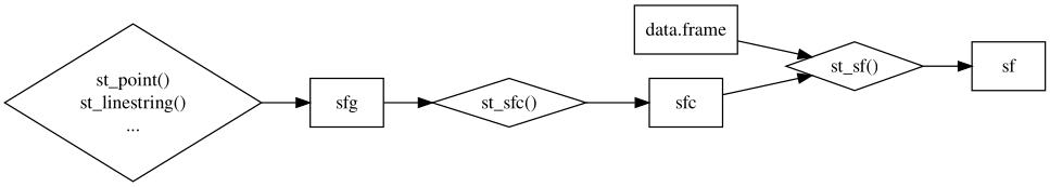
We can create sf objects with categorical and numeric attributes using the function st_sf(). Let’s show this by creating a custom dataset for three cities in Portugal.
# create a data.frame object containing the cities and their populations
city_attr <- data.frame(
  name = c("Lisboa", "Coimbra", "Porto"),
  population = c(545796, 106655, 231800)
)

# specify points as c(lon, lat) coordinates of cities
l_coord <- st_point(c(-9.1, 38.7))
c_coord <- st_point(c(-8.4, 40.2))
p_coord <- st_point(c(-8.6, 41.1))

# create a column with the specified CRS
coordinates <- st_sfc(l_coord, c_coord, p_coord, crs = "EPSG:4326")

# create `sf` object with the data.frame and the sfc
city_data <- st_sf(city_attr, geometry = coordinates)
city_dataclass(city_data)The image below illustrates the process of creating sf objects from sfc and data.frame objects, which we did above.
Now let’s suppose we want to merge city_data with data from the major rivers in Portugal that pass through those cities.
Note: These are not the actual coordinates of the rivers. The points are simulated and made so that they pass through the major cities.
# creating river data
# data.frame object
river_names = data.frame(
  river_name = c("Tejo", "Mondego", "Douro")
)

# specify points as c(lon, lat) coordinates of rivers
t_coord <- st_linestring(rbind(c(-10, 37), c(-9.1, 38.7), c(-9.1, 39.3)))
m_coord <- st_linestring(rbind(c(-8, 38.5), c(-8.4, 40.2), c(-7.8, 41.9)))
d_coord <- st_linestring(rbind(c(-8, 42),c(-8.6, 41.1), c(-8.8, 40)))

# create a column with the specified CRS
rivers <- st_sfc(t_coord, m_coord, d_coord, crs = "EPSG:4326")

# create `sf` object with the data.frame and the sfc
river_data <- st_sf(river_names, river_geometry = rivers)
plot(river_data)
One way of joining the data is to simply attach columns with cbind().
portugal_data <- cbind(city_data, river_data)
portugal_data
Another way to join datasets is through geospatial operations. These operations allow us to filter, merge, or subset dataframes based on whether points, lines, and polygons touch, intersect, or contain other geospatial objects.
For example, let’s say we don’t know which river borders which city and we want to use geospatial operations to find out. We can use st_join() to merge both datasets based on intersections. st_join() is basically a left join in which the matches are determined by the relationships between the spatial objects.
# merge city_data with river_data
pt_data <- st_join(city_data, river_data["river_name"])    # specify "river_name" to keep it in the merged dataset
pt_data
st_join() assigns the names of the rivers to the observations in which the point (i.e., city) intersects with the line (i.e., river).
Note:
st_join()drops the geometry of the second object.
Similar to st_join(), we can filter, merge, or subset sf objects with other geospatial functions. The most common types of geospatial operations are:
st_intersects()st_disjoin()st_contains()st_overlaps()st_within()
You can learn more about the different geospatial operations in the documentation of the package.
Test your Knowledge
Create a polygon with vertices (0,0), (0,3), (3,6), (6,3), (6,0). Your answer must be a sfg object.
polygon_1 <- st_...(...(...(...)))

answer_1 <- polygon_1

test_1()
Determine whether the following points are contained in the polygon with a geospatial operation.
point_1 <- st_point(c(0,0))
point_2 <- st_point(c(3,4))
point_3 <- st_point(c(3,3))
point_4 <- st_point(c(4,5))
point_5 <- st_point(c(6,6))
points <- st_sfc(point_1, point_2, point_3, point_4, point_5)Hint: you only need to run one function.
answer_2 <- st_...(...)

test_2()
Think Deeper: once you get to the correct answer of question 2, inspect the output of
answer_2. What does it mean? How is it different than the intersection of two objects?
Which of the following functions should be used to create an object with a simple feature column and other attributes?
as_data_frame()st_sfg()st_sfc()st_sf()
# Replace ... by your answer of "A", "B", "C" or "D"
answer_3 <- "..."

test_3()
What are the common coordinate inputs for geographic CRS?
c(lat, lon)c(lon, lat)c(x, y)c(y, x)
# Replace ... by your answer of "A", "B", "C" or "D"
answer_4 <- "..."

test_4()
Part 2: Hedonic Pricing with Data from Athenian Properties
In this section, we’re going to estimate the value of apartment characteristics with a hedonic pricing function for apartments located in Athens, Greece. We’ll use the geospatial datasets depmunic and properties from the package spData.
Theory
Typically, economists rely on market prices to estimate consumers’ marginal willingness to pay for a good. When the good in question is not traded in markets, economists must resort to other strategies. One of those strategies is the hedonic pricing method.
The main assumption of hedonic pricing is that the total price of a good equals the sum of the prices of its components. Using this assumption, we can deconstruct the price of a good traded in markets and attribute part of the total price to each of its non-traded component parts. For example, we can model the price of an apartment as a function of its size, view, age, location, number of bathrooms, proximity to public service, etc. If we take two apartments that are exactly equal but only differ on their view (e.g., one might be on the 2nd floor and the other on the 30th floor of the same building), their difference in price must be the added value of the view. If we have data on the prices and attributes of several apartments, we could leverage hedonic pricing to estimate how much consumers value a nice view.
Think Deeper: what are the other underlying assumptions of hedonic pricing? When might it not be appropriate to use this method to value non-traded goods?
A model for the hedonic price of an apartment could be estimated with the following regression:
\[ P_{i} = \beta_{0} + \beta_{1} Size_{i} + \beta_{2} Age_{i} + \beta_{3} Bath_{i} + \beta_{4} View_{i} + \beta_{5} Room_{i} + \beta_{6} Park_{i} + ... + \beta_{k} X_{ki} \]
where
- \(P_{i}\) is the price per square meter of apartment \(i\)
- The variables \(Size\), \(Age\), \(Bath\), \(View\), \(Room\), \(Park\), \(...\), \(X_{k}\) are the components of the apartment
- The \(\beta_{k}\)s are the effects of those components on the price of the apartment
With that in mind, let’s try to estimate the hedonic pricing function of apartments in Athens.
Exploratory Analysis
Let’s load two datasets from the spData package.
depmunichas information on the 7 districts of the municipality of Athens. The district boundaries are stored in the data as polygons.propertieshas data on properties for sale in the city of Athens. Property locations are stored in the data as points.
Let’s start with depmunic.
head(depmunic)
str(depmunic)
We can see that the dataset has attributes of the districts: airbnb, museums, population, …
We can also see that the CRS used for this dataset is a Greek CRS: Projected CRS: GGRS87 / Greek Grid. This tells us that we’re dealing with a projected CRS tailored to Greece. A quick search will find that the units of reference are in meters.
Note: a crucial part of geospatial data exploration is learning about the CRS of the dataset. This not only affects the relationships within your own dataset but also determines whether you can merge or filter geospatial objects based on other datasets.
Let’s plot the depmunic data. We specify the attribute greenspace ["greensp"] to plot a chart of the green space exclusively.
plot(depmunic["greensp"])The plot shows that the district in yellow (district 2) is the one with largest greenspace, almost 10 times as much as the district in dark blue (district 4).
Now let’s take a look at our properties data.
head(properties)
str(properties)
We can see that the dataset has attributes of the properties: size, price, age, …
We can see that the CRS used for this dataset is also the Greek CRS. This is good news: both our datasets are referenced to the same grid.
Let’s plot our properties dataset.
plot(properties["prpsqm"])The plot shows the distribution of properties with their color representing the price per square meter prpsqm. It’s hard to see a pattern from this chart, but it seems that most of the expensive properties are located towards the south.
Let’s plot our property locations on top of our district boundaries.
plot(depmunic["num_dep"], reset = FALSE)
plot(properties["price"], add = TRUE, col = "darkgreen")
Empirical Methods
Let’s try to put together a model to explain the price of properties in Athens using the hedonic pricing method. Our proposed specification will be: \[ P_{i} = \beta_0 + \beta_1 Size_{i} + \beta_2 Age_{i} + \beta_{3} Dist_{i} + \sum_{j=2}^{7} \gamma_{j} D_{ij} + \epsilon \]
where
- \(P_{i}\) is the price (in euros) per square meter of apartment \(i\),
- \(Size_{i}\) is the size in square meters of apartment \(i\),
- \(Age_{i}\) is the age in years of apartment \(i\),
- \(Dist_{i}\) is the distance between apartment \(i\) and the closest metro in meters,
- \(D_{ij}\) are dummy variables indexing the districts \(j\) for apartment \(i\).
The dummy variables are included to account for district-specific characteristics, such as the number of museums, parks, area of greenspace, and other district specific factors that we don’t have data on.
Looking at our properties dataset, we see that we already have data on all of our regressors except district location of the apartments. We need to use what we learned about geospatial operations to assign a categorical variable indicating district location to each property.
Below we use the function st_join() to merge both datasets based on the intersection of the spatial elements, and pass the attribute num_dep (the district number) to the merged dataset.
# find location districts for each property
merged_data <- st_join(properties, depmunic["num_dep"])
merged_data
Notice that st_join() dropped the district boundaries. That is fine, since num_dep already indicates where each property is located. As a matter of fact, we don’t even need the points anymore. We only needed them to connect the apartments to their district! Let’s clean our data before running our model.
Note: we should drop spatial objects with the function
st_drop_geometry(), as opposed toselect().
model_data <- merged_data %>%
                select(size, prpsqm, age, dist_metro, num_dep)%>%
                mutate(num_dep = as_factor(num_dep))%>%    # so that R understand that this is a categorical variable
                st_drop_geometry()
str(model_data)
Results and Analysis
Now, we’re ready to run our hedonic pricing model. Let’s do that using lm(). R will automatically create dummy variables for each district.
model1 <- lm(prpsqm ~ size + age + dist_metro + num_dep, data = model_data)
coeftest(model1, vcov = vcovHC)
The most significant factor contributing to the price of an apartment in Athens appears to be district location. Although age and distance to metro are statistically significant, their effects are quite small (as long as the property is not super old or super far from the closest metro). However, we do see a wide range of effects for district locations. Once we control for size, age, and distance from metro, the mere fact of being in district 4 decreases the price per square meter by over 1,000 euros! Maybe it’s the lack of greenspace that we have noted earlier…
Our model breaks down the price of an apartment as follows:
\[ P_{i} = 2352 + 4.3 Size_{i} -20 Age_{i} -0.1 Dist_{i} + \sum_{i=2}^{7} \gamma_{i} D_{i} + e \]
In which the added effects for the dummies are:
- District 2: \(-334\) euros
- District 3: \(-490\) euros
- District 4: \(-1031\) euros
- District 5: \(-822\) euros
- District 6: \(-918\) euros
- District 7: \(-653\) euros
District 1 is the base case (i.e., when all dummies equal zero), and is the most accretive location to the price of a property. That makes sense, since District 1 is the historic center of Athens.
Now, let’s look at how well our model actually predicts the price per square meter of properties. This can shed light on the appropriateness of using hedonic pricing strategies for properties in Athens.
summary(model1)$adj.r.squaredOur adjusted \(R^2\) says that our model only explains ~35% of the variation in the price of properties in Athens. The cause of low predictive power could be an error of methodology (prices of properties in Athens might not be the sum of their component parts!), or a missing variable problem.
Think Deeper: what component parts of properties might we be missing in our hedonic pricing model?